Introduction and assumptions
Borders clearly aren’t static; they change over years, decades and centuries as countries grow, shrink, and are born and die. As time passes, they may become vague or disputed. Therefore, I’d argue that you do need to create a somewhat detailed history of a region to properly map out where its borders are at a certain time. However, it should be relatively easy to get a decent idea of where a country’s borders lie when it is first formed, assuming certain conditions hold.
I’m going to suggest a way to build a country’s borders from the ground up, starting from a small city-state society with medieval or pre-medieval technology. I want to make a few key assumptions:
- Power is somewhat centrally located, preferably in a city or military fortification. This is the most secure part of the state, and it is easier to control land closer to this location than land farther away.
- Territory is contiguous; you should be able to travel from any one point to another via land while remaining in the country.
- The technology is sufficiently limited such that the above assumptions hold. While naval power may be possible, air travel is not. This should hold for the sort of society we’re talking about, assuming there aren’t significant magical powers.
- Neighboring states have relatively similar strengths. I’ll address scenarios where this isn’t true more at the end.
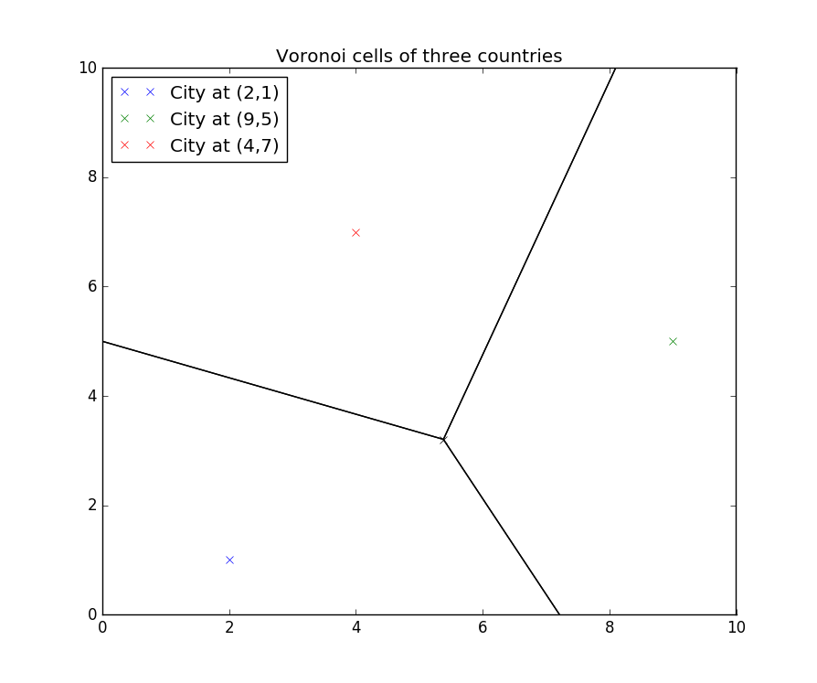
I’ll hypothesize that the original borders of a city-state, according to what I discussed above, can be approximated by creating a Voronoi diagram. Essentially, given a set of $n$ points (cities) in some two-dimensional space, a Voronoi diagram divides that space up into $n$ regions. The region $r_i$ contains all the points closer to point (city) $c_i$. The lines of the diagrams can be interpreted as the borders of these regions. Here’s an example:

Image courtesy of Wikipedia user Balu.ertl under the Creative Commons Attribution-Share Alike 4.0 International license.
Voronoi diagrams have already been used to model the borders of countries and states; see specifically the work of Jason Davies (images copyrighted, by the way). There are certainly many differences from real-life borders (although in certain parts, like North Africa, things seem to work), but again, this is only a first approximation.
For large $n$, creating such a diagram becomes a little complicated. Brute-force searches work but are obviously tedious; more sophisticated methods like Fortune’s algorithm become useful. For more information, see Easiest algorithm of Voronoi diagram to implement? and How do I derive a Voronoi diagram given its point set and its Delaunay triangulation?.
However, I’d like to deal with a much simpler case, where $n=3$. $n=1$ is obviously trivial, and $n=2$ yields precisely one border - namely, the perpendicular bisector of the line segment connecting the two cities. However, $n=3$ is a little more interesting, although it is certainly simple to solve. All we need to do is find the one vertex where all three borders coincide.
There are several ways in which we can do this, knowing the locations of three cities and assuming that each one is the center of its own city-state. We could use one of the above algorithms, if we really wanted, but those can be time-consuming to implement. Alternatively, we could use the fact that any Voronoi vertex is the center of a circle containing three points, and therefore, given three points, we could find the center of that circle. However, I’d like to use what I think is the simplest option: Determine perpendicular bisectors of segments connecting any two cities, and find the point where they intersect.
Some assumptions (well, just one, for now):
- The three points are not collinear. If they are, then the borders are just parallel lines, and there is no central vertex.
Mathematics
Let’s have a set $C$ of three cities, $(c_1(x_1,y_1),c_2(x_2,y_2),c_3(x_3,y_3))$. We choose to find the segments connecting $c_1$ and $c_2$ ($\bar{s_{12}}$) and $c_2$ and $c_3$ ($\bar{s_{13}}$). Given that the $\bar{s_{ij}}$ is the set of points equidistant to both $c_i$ and $c_j$, we can set
$$\sqrt{(x-x_i)^2+(y-y_i)^2}=\sqrt{(x-x_j)^2+(y-y_j)^2}\tag{1}$$
Simplifying eventually yields the equation
$$y=\frac{x_j-x_i}{y_i-y_j}x+\frac{x_i^2+y_i^2-x_j^2-y_j^2}{2(y_i-y_j)}\tag{2}$$
Clearly, this blows up if $y_i=y_j$, but if that’s the case, then the border simply has the equation $$x=\frac{1}{2}(x_j-x_i)$$
which is simple enough.
We do the above for all three sets of points. To find the vertex, we simply find the point where all three lines intersect, which is simple, as we can do it for any two of the lines.
Code
I wrote a program to do this in Python 3. To simplify things a bit, I’ve assumed that no two cities have the same $y$-coordinate, as that produces a line with infinite slope in $\text{(2)}$. If, for some reason, your setup includes a case like that, simply rotate the coordinate system a little so that all three points have different $y$-coordinates.
Here’s an example, with $c_1=(2,1)$, $c_2=(9,5)$ and $c_3=(4,7)$:
import numpy as np
import matplotlib.pyplot as plt

P1 = [2,1]
P2 = [9,5]
P3 = [4,7]

Set = [P1,P2,P3]

def dist(point1,point2):
    """Returns distance between two points."""
    x1 = point1[0]
    y1 = point1[1]
    x2 = point2[0]
    y2 = point2[1]
    return np.sqrt((x2 - x1)**2 + (y2 - y1)**2)

def perp(point1,point2):
    """Returns slope and y-intercept of the perpendicular
    bisector of the segment connecting two cities."""
    x1 = point1[0]
    y1 = point1[1]
    x2 = point2[0]
    y2 = point2[1]
    m = (x2 - x1)/(y1 - y2)
    b = (x1**2 + y1**2 - x2**2 - y2**2)/(2*(y1 - y2))
    return m,b

M1 = perp(P1,P2)[0]
B1 = perp(P1,P2)[1]
M2 = perp(P1,P3)[0]
B2 = perp(P1,P3)[1]
def vertex():
    """Finds central vertex"""
    x = (B1 - B2)/(M2 - M1)
    y = M1*x + B1
    return x,y

"""
This next bit divides each of the lines into a certain number of line
segments by adding a number of points onto the lines, and then removes
those points in the third city's Voronoi cell.
"""
for point1 in Set:
    for point2 in Set:
       if point2 != point1:
           N = []
           delta = 0.001
           for i in range(0,10000):
               N.append(i*delta)
           M = [perp(point1,point2)[0]*a + perp(point1,point2)[1] for a in N]
           Other_point = [a for a in Set if a not in [point1,point2]]
           i = 0
           while i < len(N):
               x = N[i]
               y = M[i]
               if dist([x,y],point1) > dist([x,y],Other_point[0]):
                   N.remove(x)
                   M.remove(y)
               else:
                   i += 1
           plt.plot(N,M,'k')

for point in Set:
    name = 'City at ('+str(point[0])+','+str(point[1])+')'
    plt.plot(point[0],point[1],'x',label=name)

plt.plot(vertex()[0],vertex()[1],'kx')
plt.legend(loc='upper left')
plt.title('Voronoi cells of three countries')
plt.xlim(0,10)
plt.ylim(0,10)
plt.show()
Here’s the output:

Approximation 2: Terrain.
Voronoi cells are, I think, a decent approximation. However, they completely ignore the landscape and terrain of the area. For instance, if an edge lies in the middle of a valley surrounded by two high mountain ranges, it seems possible that the border may shift to one of those ranges, as they’re easier to defend. The same thing goes for rivers, cliffs, etc.
I’ll assume that the following objects would cause borders to shift:
- Rivers
- Mountains
- Canyons
- Large bodies of water
I think these objects have been sufficiently justified as limitations (see celtschk ‘s answer).
Mathematics
Most of these can be approximated with curves of essentially negligible thickness (lakes and oceans aside). Therefore, let’s say that any landform $L$ can be represented as a curve parameterized by a variable $t$:
$$\mathbf{L}=\mathbf{x}_L(t)=(x_L(t),y_L(t)),\quad t_0\leq t\leq t_f$$
We can also represent a section of border $B$ as another parameterized curve, given by a parameter $s$:
$$\mathbf{B}=\mathbf{x}_B(s)=(x_B(s),y_B(s)),\quad s_0\leq s\leq s_f$$
The challenge, then, is to come up with some iterative algorithm that maps $\mathbf{B}_{n}$ to $\mathbf{B}_{n+1}$. There are probably many options out there. I chose one of the following form:
Divide $\mathbf{B}_n$ into $N$ points $\{p_{1,n},p_{2,n},\cdots,p_{N,n}\}$.
For each $p_{i,n}(x_p,y_p)$, calculate the distance to all points on $\mathbf{L}$ and choose the point on $\mathbf{L}$ that is closest, $l_{i,n}(x_l,y_l)$.
Move $p_{i,n}$ accordingly. I played around with things and decided on a certain formula:
$$dx=\frac{x_l-x_p}{1+a\cdot\text{dist}(p_{i,n},l_{i,n})},\quad dy=\frac{y_l-y_p}{1+a\cdot\text{dist}(p_{i,n},l_{i,n})}$$
$$x_{p,n+1}=x_{p,n}+dx,\quad y_{p,n+1}=y_{p,n}+dy$$
where $a$ is some scale factor and $\text{dist}(\mathbf{a},\mathbf{b})$ is the distance between two points $\mathbf{a}$ and $\mathbf{b}$.
This can be done as many times as possible. I’ve found that in many cases, even one iteration can be enough.
Code
Here’s my implementation of the above, again written in Python 3. I’ve chosen $a=0.3$:
import numpy as np
import matplotlib.pyplot as plt

scale = 0.3

RiverPath = np.linspace(0,49,1000)
def River(t):
    x = np.sqrt(t)
    y = t*np.exp(-t)
    return x,y

BorderPath = np.linspace(0,7,1000)
def Border(t):
    x = t
    y = t/4
    return x,y

def dist(y,x):
    """
    Returns closest point on the target curve to a given
    point on the border.
    """
    Set = []
    for loc in RiverPath:
       dx = x - River(loc)[0]
       dy = y - River(loc)[1]
       distance = np.sqrt(dx**2 + dy**2)
       Set.append([distance,loc])
    Set = sorted(Set, key=lambda S: S[0])
    dR = Set[0][0]
    p = Set[0][1]
    target = River(p)
    return target

def move(Q):
    """Moves each point on the border curve parameterized by Q."""
    X = []
    Y = []
    for q in Q:
       x = Border(q)[0]
       y = Border(q)[1]
       point = dist(y,x)
       point_x = point[0]
       point_y = point[1]
       mag = np.sqrt((point_x - x)**2 + (point_y - y)**2)
       dx = (point_x - x)/(1 + scale*mag)
       dy = (point_y - y)/(1 + scale*mag)
       X.append(x + dx)
       Y.append(y + dy)
    return X,Y

plt.plot(River(RiverPath)[0],River(RiverPath)[1],'b',label='River')
plt.plot(Border(BorderPath)[0],Border(BorderPath)[1],'k',label='Border')
plt.plot(move(BorderPath)[0],move(BorderPath)[1],'r')
plt.legend(loc='upper left')
plt.show()
It uses the following parameterizations:
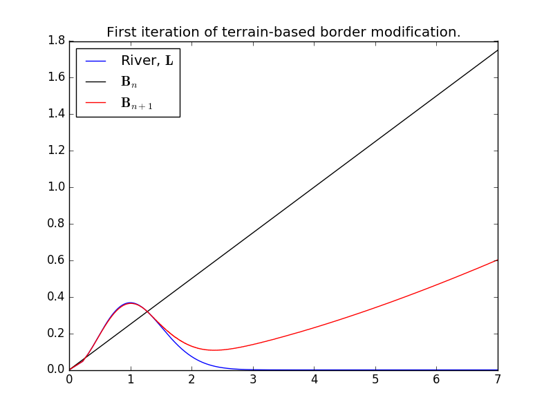
$$\mathbf{L}=(\sqrt{t},te^{-t}),\quad0\leq t\leq49,\quad\mathbf{B}_n=(s,s/4),\quad0\leq s\leq7$$
Here’s the result:

The new border hugs the river near the left, then shifts roughly halfway between the old border and the new border. More iterations might be desirable, but there’s currently something of a balance.
The formula for $dx$ and $dy$ could use some improvement, but even though it’s imperfect right now, I do think it’s functional. It can be adapted for multiple perturbing objects (i.e. multiple rivers, mountains, etc.) by calculating all the $dx$s and $dy$s, summing them, and then moving the border, not accounting for one landform at a time. You can vary the scale factor if you want, both in general and for specific landmasses. I haven’t yet played around to see how this could affect things.
Where do we go from here?
The borders of countries still don’t quite match up with these approximations. I’d argue that part of that is because of modern technology. However, a great deal is due to history. Those mountains over there are supposedly uncrossable . . . until a feud between rival kingdoms necessitates a battle, which ends with one king triumphant, ruler of both. Or maybe that river was considered a fairly good border, until holy relics were found on the other side and suddenly the head priest really wants the site inside the country.
At this point, I’d say that James’ answer becomes invaluable. In the end, it is the people of your world who shape it, often more than you, the god-like figure outside it. You can control that history, of course, but those events can and will change the world. All my suggestions are are simply slightly more detailed slates with which to start building countries. After that, it’s up to you.

